Diagnostics

Abacus exposes diagnostics through mmm.diagnostics.

Use this surface to check the design matrix, posterior sampling quality, and posterior predictive fit. For fitted-value plots and predictive sampling, see Posterior Predictive.

Diagnostic surfaces

mmm.diagnostics provides three groups of checks.

The summary methods return pandas DataFrames. The report methods return typed report objects with a to_dict() method for JSON-ready export.

Raw input screening

Use design_summary(X) on the raw design matrix you want to inspect:

design = mmm.diagnostics.design_summary(X)

By default, Abacus checks:

• all channel_columns
• all control_columns, when present

You can limit the check to specific variables:

design = mmm.diagnostics.design_summary(
    X,
    variables=["tv", "search", "price_index"],
    vif_threshold=10.0,
    near_constant_threshold=0.99,
)

The returned table includes:

• variable
• mean
• std
• n_unique
• dominant_share
• is_constant
• is_near_constant
• vif
• high_vif
• max_abs_corr

design_report(X) returns a compact roll-up with matrix rank, condition number, maximum VIF, maximum absolute correlation, and lists of flagged variables.

Screening requirements

Raw input screening requires:

• all requested columns to exist in X
• all checked columns to be numeric

Abacus raises a ValueError if a variable is missing or non-numeric.

The method names stay design_summary() and design_report(), but the pipeline now treats them as raw input screening rather than transformed model geometry.

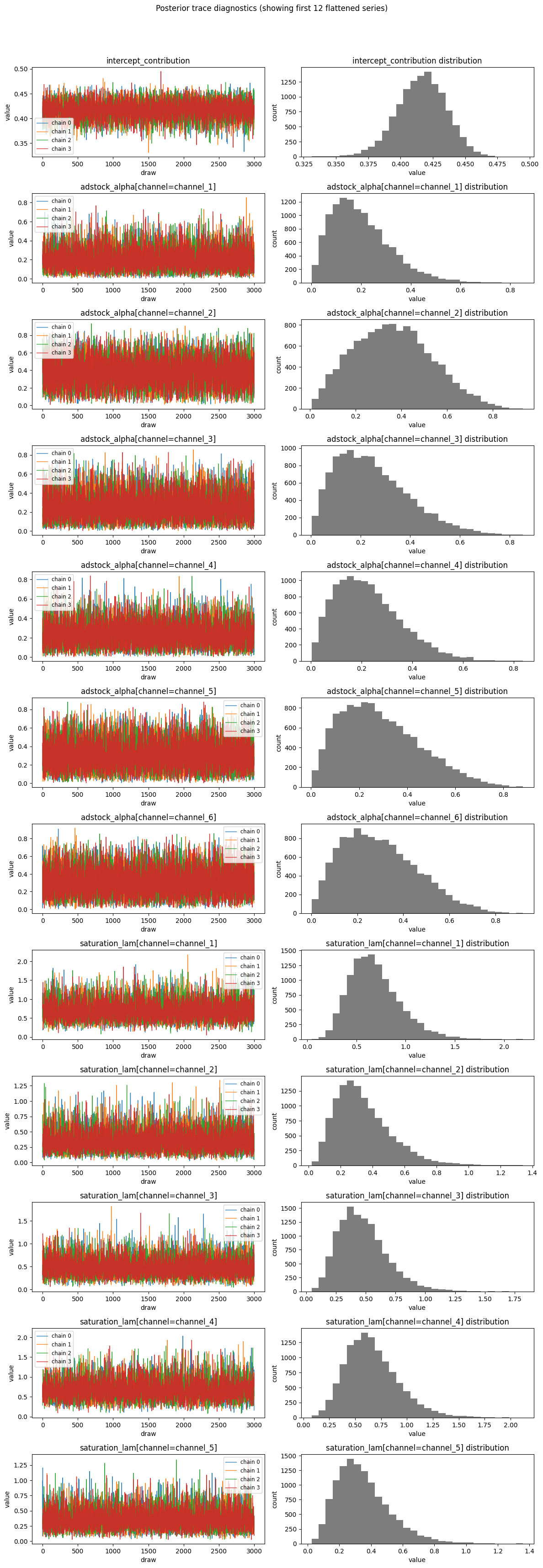
MCMC diagnostics

Use mcmc_summary() after fitting:

mcmc = mmm.diagnostics.mcmc_summary(
    rhat_threshold=1.01,
    ess_threshold=400.0,
)

The summary comes from arviz.summary(..., kind="diagnostics") and adds flag columns such as:

• high_rhat
• low_ess_bulk
• low_ess_tail

mcmc_report() adds model-level diagnostics, including:

• divergence_count
• divergence_rate
• max_rhat
• min_ess_bulk
• min_ess_tail
• bfmi_mean
• bfmi_min
• max_tree_depth_hits
• max_tree_depth_observed
• mean_acceptance_rate

If idata is missing, Abacus raises an error and tells you to fit the model first.

Example MCMC diagnostic output:

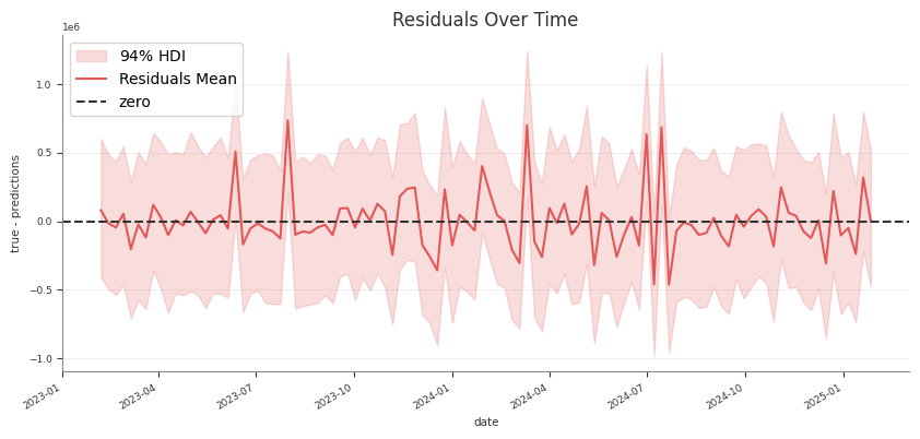
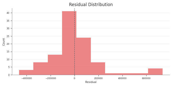
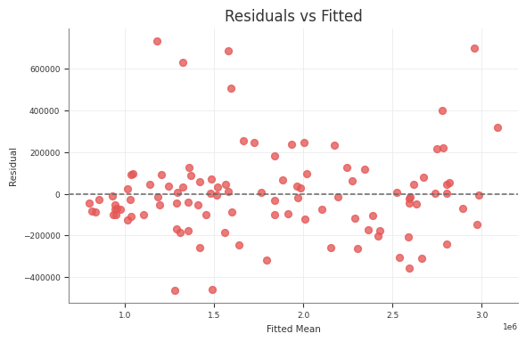
Predictive diagnostics

Predictive diagnostics use the observed target and stored posterior predictive samples:

mmm.sample_posterior_predictive(
    X=X,
    random_seed=42,
    progressbar=False,
)

predictive = mmm.diagnostics.predictive_summary(original_scale=True)

The predictive summary is a one-row DataFrame with:

• scale
• num_observations
• rmse
• mae
• nrmse
• nmae
• crps
• residual_mean
• residual_std

Abacus aligns target and prediction coordinates before flattening. That includes mixed datetime coordinate dtypes when needed.

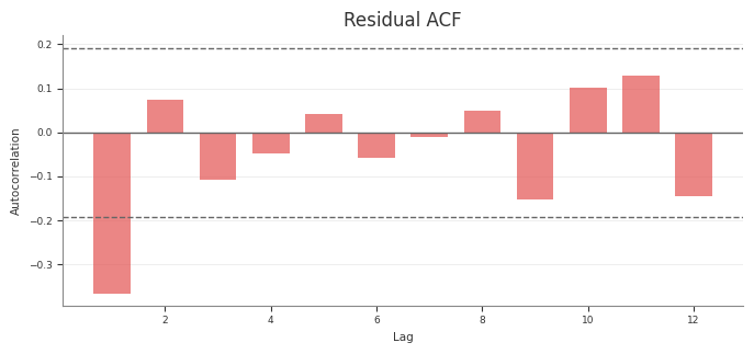
Example residual diagnostics:

Export reports

Use the report objects when you want a compact export format:

import json

report = mmm.diagnostics.mcmc_report()
payload = report.to_dict()

with open("mcmc_report.json", "w", encoding="utf-8") as handle:
    json.dump(payload, handle, indent=2)

The same pattern works for design_report(...) and predictive_report().

Pipeline outputs

The pipeline diagnostics stage uses the same retained diagnostic surfaces to write report tables and text summaries. If you run the pipeline, those stage artefacts should match the behaviour documented here.

In the structured pipeline, the raw-input screening rows in diagnostics_report.csv use the phase label raw_input_screening instead of design so the machine-readable output matches the wording here.

Common pitfalls

• Running mcmc_summary() or mcmc_report() before fitting
• Running predictive diagnostics before sampling posterior predictive values
• Passing non-numeric columns into design_summary(X)
• Treating predictive diagnostics as a substitute for design or MCMC checks