Fitting the Model

Use this page after you have prepared X and y for PanelMMM. For input requirements, see Data Preparation.

Basic workflow

fit() is the main entry point for posterior sampling.

import pandas as pd

from abacus.mmm import GeometricAdstock, LogisticSaturation
from abacus.mmm.panel import PanelMMM

dataset = pd.read_csv("data/demo/timeseries/dataset.csv")
dataset["date"] = pd.to_datetime(dataset["date"])

X = dataset.drop(columns=["revenue"])
y = dataset["revenue"].rename("revenue")

mmm = PanelMMM(
    date_column="date",
    target_column="revenue",
    channel_columns=[
        "channel_1",
        "channel_2",
        "channel_3",
        "channel_4",
        "channel_5",
        "channel_6",
    ],
    yearly_seasonality=2,
    adstock=GeometricAdstock(l_max=4),
    saturation=LogisticSaturation(),
)

idata = mmm.fit(
    X,
    y,
    draws=500,
    tune=500,
    chains=2,
    cores=2,
    progressbar=False,
    random_seed=42,
)

fit() returns an arviz.InferenceData object and also stores it on mmm.idata.

What fit() does

When you call fit(X, y), Abacus:

1. checks that pandas X and y use the same index, if both are pandas objects
2. builds the PyMC graph automatically if it has not been built already
3. merges sampler settings from the model’s sampler_config and your call-time kwargs
4. runs pymc.sample(...)
5. computes deterministic variables and adds them to the posterior group
6. stores the training data in an InferenceData.fit_data group
7. writes model metadata into idata.attrs

That means fitted contribution variables such as channel_contribution, intercept_contribution, and yearly_seasonality_contribution are available in mmm.posterior after fitting when they are part of the configured model.

Configure the sampler

You can configure PyMC sampling in two places:

Abacus merges them so that explicit fit() kwargs win.

mmm = PanelMMM(
    date_column="date",
    target_column="revenue",
    channel_columns=["channel_1", "channel_2"],
    adstock=GeometricAdstock(l_max=4),
    saturation=LogisticSaturation(),
    sampler_config={
        "draws": 1000,
        "tune": 1000,
        "chains": 4,
        "target_accept": 0.9,
        "progressbar": False,
    },
)

# Overrides draws from sampler_config, keeps target_accept
idata = mmm.fit(X, y, draws=500, random_seed=42)

Common sampler arguments

These are passed through to pymc.sample(...).

If you do not specify progressbar, Abacus defaults it to True unless your sampler_config already sets it.

When to build first

For a standard workflow, call fit() directly.

Call build_model(X, y) first only when you need to inspect or modify the graph before sampling. For example:

mmm.build_model(X, y)
mmm.add_original_scale_contribution_variable(
    var=["channel_contribution", "y"]
)

idata = mmm.fit(
    X,
    y,
    draws=500,
    tune=500,
    chains=2,
    progressbar=False,
    random_seed=42,
)

This pattern is also useful when you need to add events before fitting. Call add_events(...) before build_model(...) or fit(...).

Inspect fitted results

After fitting, common entry points are:

• mmm.idata
• mmm.posterior
• mmm.model
• mmm.plot
• mmm.summary
• mmm.diagnostics

Example:

posterior = mmm.posterior
channel_mean = posterior["channel_contribution"].mean(dim=["chain", "draw"])

Common pitfalls

• Leaving the target column inside X
• Passing pandas X and y with different indexes
• Changing the model graph after fitting and expecting existing samples to stay valid
• Assuming constructor sampler_config overrides explicit fit() kwargs; it does not
• Adding events after the model has already been built

Next steps

• Run Prior Predictive Checks before posterior sampling when you are tuning priors or model structure.
• Read Save and Load if you want to persist a fitted model.

Prior Predictive Checks

Run prior predictive checks before fitting when you want to test whether your configured priors imply plausible target behaviour.

If you want the econometrics framing for this workflow, see Prior Predictive Checks for Econometricians.

Sample prior predictive draws

Use sample_prior_predictive(...) on PanelMMM:

prior = mmm.sample_prior_predictive(
    X=X,
    y=y,
    samples=100,
    random_seed=42,
)

In normal PanelMMM use, pass the same X and y structure that you plan to fit.

sample_prior_predictive(...):

• builds the model if it has not been built yet
• samples from pymc.sample_prior_predictive(...)
• stores prior and prior_predictive on mmm.idata by default
• returns an extracted xarray.Dataset of prior predictive draws

How many draws Abacus uses

If you do not pass samples=..., Abacus uses:

• sampler_config["draws"] when that key exists
• otherwise 500

If you want prior predictive checks to use a different sample count from model fitting, pass samples explicitly.

Plot prior predictive draws

After sampling, you can use the retained plotting surface:

figure, axes = mmm.plot.prior_predictive(
    var=mmm.output_var,
    hdi_prob=0.85,
)

You can then access the stored groups directly:

prior_group = mmm.prior
prior_predictive_group = mmm.prior_predictive

Trying to access these groups before sampling raises a runtime error.

Example prior predictive output:

What to inspect

A useful prior predictive check is about plausibility, not fit.

Check:

• scale: are draws on roughly the same order of magnitude as the observed target?
• support: do the draws violate obvious business constraints such as non-negativity?
• volatility: do the draws imply far more or far less variation than the real series?
• structure: do the trajectories look broadly plausible for the business and model configuration?

If the prior predictive distribution is implausible, change the model before you fit it.

Adjust the model before fitting

Typical changes include:

• tightening intercept or likelihood priors in model_config
• revising media transformation priors
• reducing unnecessary model flexibility
• checking whether your scaling choices make priors too loose on the model scale

See Priors and Configuration for the configuration surface.

Prior predictive before and after fit

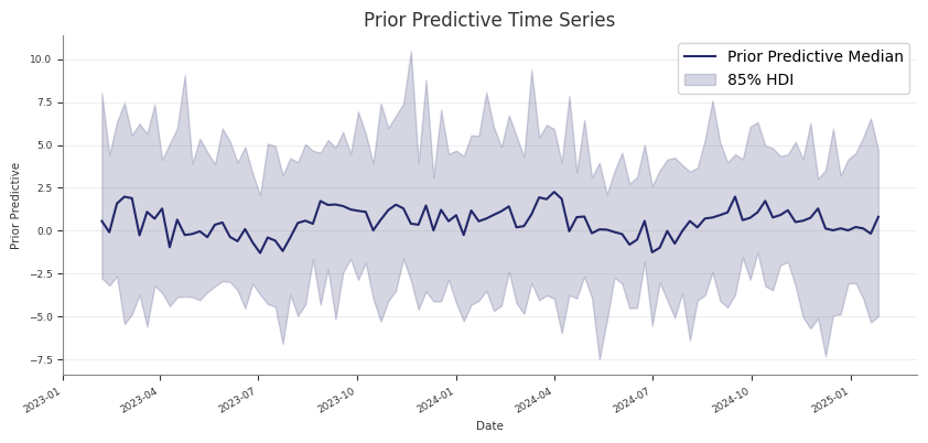
If you run prior predictive checks first and then call fit(), Abacus keeps the existing prior and prior_predictive groups on mmm.idata.

That makes it practical to compare:

• prior assumptions
• posterior fit
• posterior predictive behaviour

within one saved InferenceData object.

Common pitfalls

• Skipping prior predictive checks and only noticing implausible priors after a long fit
• Treating prior predictive checks as a substitute for posterior predictive assessment
• Forgetting that sample_prior_predictive(...) returns extracted predictive draws, while the full prior and prior_predictive groups are stored on mmm.idata

Next steps

After the prior predictive behaviour looks reasonable, fit the model with Fitting the Model.

Save and Load

Use save and load when you want to persist a fitted PanelMMM and rebuild it later without redefining the whole model configuration in code.

Basic round trip

The standard workflow is:

mmm.fit(
    X,
    y,
    draws=500,
    tune=500,
    chains=2,
    progressbar=False,
    random_seed=42,
)

mmm.save("mmm.nc")

loaded = PanelMMM.load("mmm.nc")

save() writes the model’s InferenceData to NetCDF. load() reads that file, recreates the PanelMMM configuration from stored metadata, restores loaded.idata, and rebuilds the PyMC graph from the saved training data.

What Abacus stores

Abacus relies on more than the posterior draws for a full round trip.

The stored attrs include both the shared model metadata and PanelMMM-specific configuration such as:

• date_column
• channel_columns
• target_column
• target_type
• dims
• control_columns
• control_impacts
• adstock and saturation
• adstock_first
• yearly_seasonality
• time_varying_intercept and time_varying_media
• scaling
• model_config
• sampler_config
• serialised mu_effects

save() behaviour

save(fname, **kwargs) is a thin wrapper over self.idata.to_netcdf(...).

Important constraints:

• the model must already be fitted
• self.idata must contain a posterior group
• any extra kwargs are passed directly to InferenceData.to_netcdf(...)

If you call save() before fitting, Abacus raises:

RuntimeError: The model hasn't been fit yet, call .fit() first

load() and compatibility checks

By default, PanelMMM.load(...) validates that the saved file matches the current model class and configuration:

loaded = PanelMMM.load("mmm.nc", check=True)

With check=True, Abacus verifies:

• the saved model version
• the saved model id derived from the serialised configuration

If those checks fail, Abacus raises DifferentModelError.

If you need to bypass those checks, you can set check=False:

loaded = PanelMMM.load("mmm.nc", check=False)

Use that only when you understand why the saved metadata does not match.

Load from an in-memory InferenceData

If you already have an InferenceData object, use load_from_idata(...) instead of saving to disk first:

loaded = PanelMMM.load_from_idata(idata, check=True)

This is the same round-trip path that load() uses internally after reading the NetCDF file.

Where build_from_idata() fits

build_from_idata(idata) is the lower-level rebuild step. It:

1. restores supported serialised mu_effects
2. reads idata.fit_data
3. splits that saved training data back into X and y
4. rebuilds the PyMC graph

You usually do not need to call build_from_idata() yourself because load() and load_from_idata() already do it.

Round-trip limitations

Not every fitted object can be restored fully.

EventAdditiveEffect does not round-trip

Abacus does not deserialize EventAdditiveEffect because the original df_events DataFrame is not stored in the saved attrs. In that case, PanelMMM.load(...) fails fast while rebuilding the model.

Do not drop fit_data if you want to reload

Because rebuild uses idata.fit_data, do not save a partial file that omits that group if you want to call PanelMMM.load(...) later.

For example, this is valid NetCDF output:

mmm.save("posterior_only.nc", groups=["posterior"])

But it is not a full PanelMMM round-trip artefact, because the saved file no longer includes the training data needed for build_from_idata(...).

Practical advice

• Use the default save() behaviour for round trips.
• Keep check=True unless you have a specific compatibility reason not to.
• Prefer PanelMMM.load(...) over loading NetCDF manually.
• Refit or rebuild event effects explicitly rather than expecting saved event state to deserialize.

Next steps

After loading a model, you can go straight to posterior predictive sampling, diagnostics, decomposition, or optimisation using the restored idata and rebuilt graph.